technical-interview-prep

Technical Interview Prep

Here are the sections:

• How to Succeed in Data Structures and Algorithms Interview
• Algorithms
• Data Structures
• Curated LeetCode Questions
• AlgoExpert
• Software Engineering
• System Design

These are the best online resources that I used while preparing for technical coding interviews:

• Cracking The Coding Interview: The most popular book on the whole tech interview process, now in 6th edition. 189 programming interview questions are included, ranging from the basics to the trickiest algorithm problems.
• Elements of Programming Interviews: Another great book written by professional software engineers, with different versions in C++, Java and Python.
• HackerRank: A technical recruiting platform that assesses developers based on actual coding skills.
• Pramp: A free online peer-to-peer platform for practicing technical interviews.
• LeetCode: One of the best online resource providing a rich library of more than 300 real coding interview questions with 7 supported languages - C, C++, Java, Python, C#, JavaScript, Ruby.
• Interview Cake: Another site that preps software engineering candidates for coding interview.
• AlgoExpert: The ultimate resource to prepare for coding interviews. Everything you need, in one streamlined platform.
• Software Engineering Interview Preparation: All the required theoretical material needed to pass a Facebook/Google software engineering interview.

How to Succeed in Data Structures and Algorithms Interview

To practice your algorithmic coding, review this interview preparation document.

• Preparation
• Understand the Problem
• Brute Force Solution
• Optimize Your Solution
• Code Your Solution
• Test Your Solution

Preparation

• Develop a deep knowledge of data structures: You should understand and be able to talk about different data structures and their strengths, weaknesses, and how they compare to each other. Taking the time to implement data structures from scratch will leave you much better prepared for DS&A interviews, than studying them as an abstract concept.
• Understand Big O notation: You should be able to talk about Big O notation for both time and space complexity. Make sure to read about common algorithms and their memory and runtime complexity to train your big O analysis muscle.
• Know the major sorting algorithms: Given that differences in time and space complexity can derail your optimal solution for an algorithm problem, it’s good to be familiar with the major algorithms per category (string matching, sorting, search, graph, traversal, etc).

back to current section

Understand the Problem

• To verify your understanding, repeat the question back to the interviewer in your own words to make sure you got it correctly. There’s nothing worse than realizing mid-interview that you’re answering a completely different question. It could be helpful to use a test or two to verify your understanding of the problem.
• You should feel comfortable asking your interviewer questions to define any ambiguities and ask them if you can make certain assumptions (e.g. “Can I assume the array is sorted?” or “Can I assume the input is valid?”). Remember that the interviewer’s goal is to get a good signal for how you think through an issue or problem.
• You may consider asking them the following questions:
  • How large is the range of values? What kind of values exists?
  • How large is the size of the input? Are there duplicates within the input?
  • What are some extreme cases of inputs?
  • How is the input stored?
• You should also ask whether you’ll eventually be optimizing for time, space, or both. Even if you believe you already know how to solve the problem, it’s important to ensure that you’re spending your time implementing the solution that your interviewer cares about.
• Keep track of how much time you’re spending in the ideation phase to leave yourself enough time to code your solution.

back to current section

Brute Force Solution

• The worst outcome in a technical interview is to not write any code, and the easiest way to end up in that position is to overcomplicate the problem early in the interview.
• Instead, talk through a solution you’re confident will work and let your interviewer know about the concessions you’ve made. You might think that if you present an initial suboptimal solution that you’ll never get hired, but this isn’t true. Communication is important here. You can score points with your interviewer by explaining the time and space complexity of your naive or brute-force solution and by clarifying why it’s suboptimal; you’ll have the chance to improve it later.
• Now that you’ve talked through the brute-force solution, ask the interviewer whether they’d like you to implement the brute force solution or come up with a more efficient solution. If the former, skip the next section “Optimize your Solution” and come back to it at the end. Only start coding once you and your interviewer have agreed on an approach and they’ve given you the green light to move ahead.

back to current section

Optimize Your Solution

• Discuss your approach with your interviewer and lean on them to get a sense of whether they have a preference for whether you optimize for time, space, or both. When optimizing, some of your initial assumptions may change, so it’s important to check with your interviewer.
• You may see the most optimal solution right away or be unsure on how to proceed. If you’re stuck, here are some common approaches to optimizing:
  • Take a second look at the problem, its constraints, and write down your assumptions and possible simplifications.
  • Consider similar problems you’ve seen and discuss them with your interviewer.
  • Solve an example by hand and extrapolate about what algorithm(s) could be used.
  • Simulate the brute-force solution by hand and identify the inefficiencies that could be optimized with a data structure.
  • Solve a simple version of the problem first, then build on it.
• Don’t forget to communicate and analyze the time or space complexity of the solution you plan to optimize. Once you and your interviewer agree that you have a good solution, it’s time to code it.

back to current section

Code Your Solution

• As an interviewee, it’s important to ensure that your interviewer understands what you’re doing and why you’re doing it in real-time. If you’re explaining your thought process out loud and you take a wrong turn, your interviewer may offer you a hint to get you back on track.
• While you’re coding, don’t read your code verbatim; but rather, talk about the section of the code you’re implementing at a higher level. Explain why you wrote it that way and what it’s trying to achieve.
• Remember that your interviewer needs to be able to understand your code to efficiently evaluate whether your code returns the expected result and solves the problem. As you code, keep these pointers in mind:
  • Use good style when writing your code.
  • Naming Matters.
  • Demonstrate good modularity.
  • Leave time to check for bugs and edge cases.
  • If cutting corners, explain it to your interviewer.
• Take a step back and briefly read through your solution, examining it as if it were written by someone else, but don’t start debugging it manually. This is the same approach that will be taken by your interviewer. Fix any issues you may find.
• Then walk your interviewer through the code and explain your rationale. If you find a bug or mistake, feel free to acknowledge it and make the change.

back to current section

Test Your Solution

• During the testing portion of the interview, you should have a few goals in mind. You want to…
  • Demonstrate that you care that your code actually works.
  • Show that you can understand and solve problems even if it doesn’t work.
  • Exhibit your understanding of the various edge cases that a real-world problem might present.
  • Establish a feedback loop for your code that allows refactoring without having to worry about breaking existing functionality.
• There are a few types of inputs you’re going to test for:
  • Large and small valid inputs.
  • Large and small invalid inputs.
  • Random input.
• For each input, manually go through your code and ensure that it performs. You should jot down or tell your interviewer the values of each variable as you walk them through the code.
• If you find an error, explain the error to your interviewer, fix it, and move on. Similarly, if there are large duplicated code blocks in your solution, you can take the time to restructure the code.
• In this stage, you’ll also have the opportunity to showcase your knowledge around automated testing. You can chat about how you’d generate different types of inputs, how you would stub parts of the code, the test runners you’d use, and more. These are all great signals to show an interviewer.

back to current section

back to top

Algorithms

Here are the algorithms:

• Sorting
• Tree Traversals
• Graph Traversals
• Backtracking
• Binary Search
• Breadth First Search
• Depth First Search
• Recursion

Sorting

Bubble Sort

• This simple sorting algorithm iterates over a list, comparing elements in pairs and swapping them until the larger elements “bubble up” to the end of the list, and the smaller elements stay at the “bottom”.
• Implementation
• In the worst case scenario (when the list is in reverse order), this algorithm would have to swap every single item of the array. Therefore, if we have n elements in our list, we would have n iterations per item - thus Bubble Sort’s time complexity is O(n^2).

Selection Sort

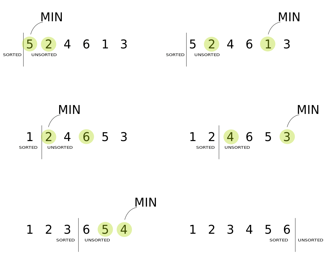
• This algorithm segments the list into two parts: sorted and unsorted. We continuously remove the smallest element of the unsorted segment of the list and append it to the sorted segment.
• Implementation
• For a list with n elements, the outer loop iterates n times. The inner loop iterate n-1 when i is equal to 1, and then n-2 as i is equal to 2 and so forth. The amount of comparisons are (n - 1) + (n - 2) + ... + 1, which gives Selection Sort a time complexity of O(n^2).

Insertion Sort

• Like Selection Sort, this algorithm segments the list into sorted and unsorted parts. It iterates over the unsorted segment, and inserts the element being viewed into the correct position of the sorted list.
• Implementation
• In the worst case scenario, an array would be sorted in reverse order. The outer for loop in Insertion Sort function always iterates n-1 times. In the worst case scenario, the inner for loop would swap once, then swap two and so forth. The amount of swaps would then be 1 + 2 + ... + (n - 3) + (n - 2) + (n - 1) which gives Insertion Sort a time complexity of O(n^2).

Heap Sort

• This popular sorting algorithm, like the Insertion and Selection sorts, segments the list into sorted and unsorted parts. It converts the unsorted segment of the list to a Heap data structure, so that we can efficiently determine the largest element.
• Implementation
• Let’s first look at the time complexity of the heapify function. In the worst case the largest element is never the root element, this causes a recursive call to heapify. While recursive calls might seem dauntingly expensive, remember that we’re working with a binary tree. Visualize a binary tree with 3 elements, it has a height of 2. Now visualize a binary tree with 7 elements, it has a height of 3. The tree grows logarithmically to n. The heapify function traverses that tree in O(log(n)) time.
• The heap_sort function iterates over the array n times. Therefore the overall time complexity of the Heap Sort algorithm is O(nlog(n)).

Merge Sort

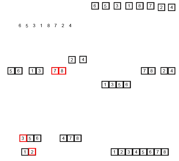
• This divide and conquer algorithm splits a list in half, and keeps splitting the list by 2 until it only has singular elements. Adjacent elements become sorted pairs, then sorted pairs are merged and sorted with other pairs as well. This process continues until we get a sorted list with all the elements of the unsorted input list.
• Implementation
• Let’s first look at the merge function. It takes two lists, and iterates n times, where n is the size of their combined input.
• The merge_sort function splits its given array in 2, and recursively sorts the sub-arrays. As the input being recursed is half of what was given, like binary trees this makes the time it takes to process grow logarithmically to n. Therefore the overall time complexity of the Merge Sort algorithm is O(nlog(n)).

Quick Sort

• This divide and conquer algorithm is the most often used sorting algorithm. When configured correctly, it’s extremely efficient and does not require the extra space Merge Sort uses. We partition the list around a pivot element, sorting values around the pivot.
• Implementation
• The worst case scenario is when the smallest or largest element is always selected as the pivot. This would create partitions of size n-1, causing recursive calls n-1 times. This leads us to a worst case time complexity of O(n^2).
• While this is a terrible worst case, Quick Sort is heavily used because it’s average time complexity is much quicker. While the partition function utilizes nested while loops, it does comparisons on all elements of the array to make its swaps. As such, it has a time complexity of O(n).
• With a good pivot, the Quick Sort function would partition the array into halves which grows logarithmically with n. Therefore the average time complexity of the Quick Sort algorithm is O(nlog(n)).

Time Complexities of All Sorting Algorithms

back to current section

Tree Traversals

Tree traversals are commonly used in interviews. Learn about pre-order, in-order and post-order traversal in this video.

• Often we want to visit the nodes of a tree in a particular order (for example, print the nodes of the tree)
• Depth-First: We completely traverse one sub-tree before exploring a sibling sub-tree (pre-oder, in-order, post-order).
• Breadth-First: We traverse all nodes at one level before progressing to the next level.
• When working with a tree, recursive algorithms are common.

Depth-First

InOrderTraversal(tree)

if tree = nil: return
InOrderTraversal(tree.left)
Print(tree.key)
InOrderTraversal(tree.right)

PreOrderTraversal(tree)

if tree = nil: return
Print(tree.key)
PreOrderTraversal(tree.left)
PreOrderTraversal(tree.right)

PostOrderTraversal(tree)

if tree = nil: return
PostOrderTraversal(tree.left)
PostOrderTraversal(tree.right)
Print(tree.key)

Breadth-First

LevelTraversal(tree)

if tree = nil: return
Queue q
q.Enqueue(tree)
while not q.Empty():
  node <- q.Dequeue()
  Print(node)
  if node.left != nil:
    q.Enqueue(node.left)
  if node.right != nil:
    q.Enqueue(node.right)

back to current section

Graph Traversals

• The process of searching through or traversing through a graph data structure involves visiting each vertex/node in a graph. The order in which vertices are visited is how we can classify graph traversals.
• A Quick Review:
  • BFS traverses broad into a structure by visiting sibling/neighbor nodes before children nodes. It uses a queue data structure.
  • DFS: traverses deep into a structure by visiting children nodes before visiting sibling/neighbor nodes. It uses a stack data structure.
• Graph traversal can begin with any node, since there is no concept of a root node.

BFS Traversal

• A unique thing about BFS is that it lends itself quite nicely to determining the shortest path between any node in the graph and the “parent” node.
  • In fact, most BFS implementations will keep track of every single node’s “parent” nodes that come before it.
  • This is helpful because we can use the pointers of the path that we take to get to a node from the starting node in order to determine a shortest path in the graph.
• The power of using breadth-first search to traverse through a graph is that it can easily tell us the shortest way to get from one node to another.
• If we must visit every node once, and check every edge in its adjacency list, the runtime complexity for both a directed and undirected graph is the sum of the vertices and their edges as represented by the graph in its adjacency list representation, or O(V + E).

DFS Traversals

• While BFS will traverse through a graph one level of children at a time, DFS will traverse down a single path, one child node at a time.
  • BFS is good to find a shortest path.
  • DFS tells us if a path even exists.
• DFS is like solving a maze:
  • We’ll continue to walk through the path of the maze until we reach a dead end.
  • When we do reach a dead end, we backtrack until we find another path we haven’t walked yet, and repeat.
  • Eventually, we will be able to determine if we can get out of the maze.
• DFS requires O(V + E) runtime:
  • For a directed graph, |E| edges to check.
  • For an undirected graph, 2|E| edges (each edge is visited twice).

Pros and Cons

• DFS:
  • Not helpful in finding shortest paths. We could end up following the longest path from node x to y!
  • But if the graph is deep enough, it can be great since we don’t need to store the entire thing in memory!
• BFS:
  • Can be great to find the shortest path possible.
  • But if the graph is wide, we’d need to store all of it, level by level, with references and using memory unnecessarily!

back to current section

Backtracking

Learn about backtracking in this video:

• Backtracking solves problems by trying a series of actions. If a series fails, we back up and try a different series.
• A maze is a classic example, but the approach can be used on a wide variety of problems.
• The recursive solution may be elegant, but remember not to dwell on the backtracking concept or what the recursion is doing.

back to current section

Binary Search

Binary search is an efficient algorithm for finding an item from a sorted list of items. It works by repeatedly dividing in half the portion of the list that could contain the item, until you’ve narrowed down the possible locations to just one.

We basically ignore half of the elements just after one comparison.

1. Compare x with the middle element.
2. If x matches with middle element, we return the mid index.
3. Else If x is greater than the mid element, then x can only lie in right half subarray after the mid element. So we recur for right half.
4. Else (x is smaller) recur for the left half.

Recursive and Iterative Implementation

back to current section

Breadth First Search

Breadth First Search (BFS) is a widely used interview question. Learn about it in this video. It is an algorithm used for tree traversal on graphs or tree data structures. BFS can be easily implemented using recursion and data structures like dictionaries and lists.

The Algorithm

1. Pick any node, visit the adjacent unvisited vertex, mark it as visited, display it, and insert it in a queue.
2. If there are no remaining adjacent vertices left, remove the first vertex from the queue.
3. Repeat step 1 and step 2 until the queue is empty or the desired node is found.

• Implementation
• Since all of ​the nodes and vertices are visited, the time complexity for BFS on a graph is O(V + E); where V is the number of vertices and E is the number of edges.

back to current section

Depth First Search

Depth First Search (DFS) is a widely used interview question. Learn about it in this video. It is an algorithm for tree traversal on graph or tree data structures. It can be implemented easily using recursion and data structures like dictionaries and arrays.

The Algorithm

1. Pick any node. If it is unvisited, mark it as visited and recur on all its adjacent nodes.
2. Repeat until all the nodes are visited, or the node to be searched is found.

• Implementation
• Since all of ​the nodes and vertices are visited, the time complexity for DFS on a graph is O(V + E); where V is the number of vertices and E is the number of edges. In case of DFS on a tree, the time complexity is O(V), where V is the number of nodes.

back to current section

Recursion

Learn about recursion in this video:

• Used when problems exhibit common sub-structures.
• SumUpTo(n): Base case = 1 when n = 1; Recursive/Inductive case = n + SumUpTo(n - 1) when n > 1

def sum_up_to(n):
  if n == 1: return 1
  else: return n + sum_up_to(n - 1)

def is_palindrome(word):
  if len(word) < 2: return True
  else:
    if word[0] != word[-1]: return False
    else: return is_palindrome(word[1:-1])

back to current section

back to top

Data Structures

Here are the most commonly used data structures:

1. Arrays
2. Stacks
3. Queues
4. Linked Lists
5. Trees
6. Graphs
7. Hash Tables
8. Set
9. Heaps
10. Tries
11. Comparisons

Arrays

An array is the simplest and most widely used data structure. Other data structures like stacks and queues are derived from arrays.

Here’s an image of a simple array of size 4, containing elements (1, 2, 3 and 4).

Each data element is assigned a positive numerical value called the ≈Index**, which corresponds to the position of that item in the array. The majority of languages define the starting index of the array as 0.

Basic Operations on Arrays:

• Insert — Inserts an element at given index: O(n)
• Get — Returns the element at given index: O(n)
• Delete — Deletes an element at given index: O(n)
• Size — Get the total number of elements in array: O(1)

Commonly Asked Array Interview Questions:

1. Find the second minimum element of an array

• A simple solution is to sort the array in increasing order. The first 2 elements in sorted array would be 2 smallest elements. Time complexity is O(n logn).
• A better solution is to scan the array twice. In 1st traversal, find the minimum element. Let this element be x. In 2nd traversal, find the smallest element greater than x. Time complexity of this solution is O(n).
• An efficient solution can find the minimum 2 elements in one traversal.

1> Initialize both first and second smallest as INT_MAX
2> Loop through all elements:
  a> If the current element is smaller than the first, then update first and second.
  b> Else if the current element is smaller than second, then update second.

2. Find the first non-repeating element in an array of integers

• A simple solution is to use 2 loops. The outer loop picks elements one by one and inner loop checks if the element is present more than once or not.
• An efficient solution is to use hashing: (1) Traverse array and insert elements and their counts in a hash table. (2) Traverse array again and print first element with count equals to 1.
• Further optimization: If array has many duplicates, we can also store index in hash table, using a hash table where value is a pair. Now we only need to traverse keys in hash table to find first non-repeating.

3. Merge two sorted arrays

• The idea is to use Merge function of Merge sort - O(n1 + n2) time and O(n1 + n2) space
  • Create a new array arr3[] of size n1 + n2.
  • Simultaneously traverse arr1[] and arr2[]
    • Pick smaller of current elements in arr1[] and arr2[], copy this smaller element to next position in arr3[] and move ahead in arr3[] and the array whose element is picked.
  • If there are remaining elements in arr1[] or arr2[], copy them also in arr3[].

4. Remove even integers from an array

back to current section

Stacks

• A real-life example of Stack could be a pile of books placed in a vertical order. In order to get the book that’s somewhere in the middle, you will need to remove all the books placed on top of it. This is how the LIFO (Last In First Out) method works.
• Stacks are often implemented by using a linked list! Because they can only “grow” in one direction — that is to say, they only allow us to add and remove elements through a single place — they lend themselves easily to behaving exactly like singly linked lists.
• If we remember the characteristics of a linked list, we’ll recall that they have a head node, and that the space time complexity of adding elements to the beginning of the linked list is O(1), or constant time. That’s really nice, because no matter how big our stack might get, since we’re only adding and removing from the top (our head node), we can perform that single operation in relatively the same amount of time, even with a large stack.
• What happens when you implement a stack using an array as our data structure? Well, if we try to add more elements to our stack than our array has space for…things turn real bad, real fast. Our stack won’t prevent us from adding another element (since it thinks that it can grow as large as it wants), but the array that’s implementing the stack won’t have the space that’s required to allocate enough memory to the new element that we’re adding! All of this leads to — you guessed it — a stack overflow!

Here’s an image of stack containing three data elements (1, 2 and 3), where 3 is at the top and will be removed first:

Basic Operations of Stack:

• Push — Inserts an element at the top: O(1)
• Pop — Returns the top element after removing from the stack: O(1)
• isEmpty — Returns true if the stack is empty: O(1)
• Top — Returns the top element without removing from the stack: O(1)

class Stack:

    def __init__(self):
        self.stack = []

    def add(self, dataval):
        # Use list append method to add element
        if dataval not in self.stack:
            self.stack.append(dataval)
            return True
        else:
            return False

    def peek(self):
        # Use peek to look at the top of the stack
	       return self.stack[-1]

    def remove(self):
        # Use list pop method to remove element
        if len(self.stack) <= 0:
            return ("No element in the Stack")
        else:
            return self.stack.pop()

Commonly Asked Stack Interview Questions:

1. Implement two stacks using one array

2. Sort values in a stack

3. Check balanced parentheses in an expression

back to current section

Queues

• Similar to Stack, Queue is another linear data structure that stores the element in a sequential manner. The only significant difference between Stack and Queue is that instead of using the LIFO method, Queue implements the FIFO method, which is short for First in First Out.
• A perfect real-life example of Queue: a line of people waiting at a ticket booth. If a new person comes, they will join the line from the end, not from the start — and the person standing at the front will be the first to get the ticket and hence leave the line.
• Arrays can be very powerful when we know the size of our data structure ahead of time. But there a many times (in particular with queues) when we don’t really know how big our queue is going to get. So what happens when we have to enqueue an element? Well, if we don’t know the queue size beforehand and we’re using an array, it’s probable that sooner rather than later, we’ll run out of allocated memory and space. So, we’ll need to copy over the contents of our array and then allocate more space and memory, and then enqueue a new element onto the end of the queue.
• But there’s yet another added complexity with array-based queue implementations: we need to be able to enqueue at the back of the array, and dequeue from the front — which isn’t always terrible because accessing the first or last element in an array doesn’t take too much time, but it’s not as simple as with stacks, where the adding and removing of elements all happens from one end of the structure. As our array grows, we’ll need to be able to access one end and the other, and the space time complexity will grow as a result.
• We can implement the queue with a linked list. We don’t need to worry about the queue size ahead of time, since memory can be distributed and the linked list implementation of our queue can grow dynamically (just as long as we don’t use all of our computer’s memory).
• Enqueuing and dequeuing gets to be a lot easier, because we can simply find an empty space in memory, add a node with a reference to it’s next neighbor. No need to copy and recreate our queue like we had to with an array implementation. And, if we add pointer references to the beginning and end of our list, we don’t need to traverse the entire structure to enqueue or dequeue an element, either!

Here’s an image of Queue containing four data elements (1, 2, 3 and 4), where 1 is at the top and will be removed first:

Basic Operations of Queue:

• Enqueue() — Inserts element to the end of the queue: O(1)
• Dequeue() — Removes an element from the start of the queue: O(1)
• isEmpty() — Returns true if queue is empty: O(1)
• Top() — Returns the first element of the queue: O(1)

A queue can be implemented using python list where we can use the insert() and pop() methods to add and remove elements. Their is no insertion as data elements are always added at the end of the queue.

class Queue:

    def __init__(self):
        self.queue = list()

    def addtoq(self,dataval):
        # Insert method to add element
        if dataval not in self.queue:
            self.queue.insert(0,dataval)
            return True
        return False

    def size(self):
        return len(self.queue)

    # Pop method to remove element
    def removefromq(self):
        if len(self.queue)>0:
            return self.queue.pop()
        return ("No elements in Queue!")

Commonly Asked Queue Interview Questions:

1. Implement stack using a queue

2. Reverse first k elements of a queue

3. Generate binary numbers from 1 to n using a queue

back to current section

Linked Lists

• A linked list is another important linear data structure which might look similar to arrays at first but differs in memory allocation, internal structure and how basic operations of insertion and deletion are carried out.
• A linked list is like a chain of nodes, where each node contains information like data and a pointer to the succeeding node in the chain. There’s a head pointer, which points to the first element of the linked list, and if the list is empty then it simply points to null or nothing.
• Linked lists are used to implement file systems, hash tables, and adjacency lists.

Here’s a visual representation of the internal structure of a linked list:

Following are the types of linked lists:

• Singly Linked List (Unidirectional)
• Doubly Linked List (Bi-directional)

Basic Operations of Linked List:

• InsertAtEnd — Inserts given element at the end of the linked list: O(1)
• InsertAtHead — Inserts given element at the start/head of the linked list: O(1)
• Delete — Deletes given element from the linked list: O(1)
• DeleteAtHead — Deletes first element of the linked list: O(1)
• Search — Returns the given element from a linked list: O(n)
• isEmpty — Returns true if the linked list is empty: O(1)

A good rule of thumb for remember the characteristics of linked lists is this: a linked list is usually efficient when it comes to adding and removing most elements, but can be very slow to search and find a single element.

• If you ever find yourself having to do something that requires a lot of traversal, iteration, or quick index-level access, a linked list could be your worst enemy. In those situations, an array might be a better solution, since you can find things quickly (a single chunk of allocated memory), and you can use an index to quickly retrieve a random element in the middle or end of the list without having to take the time to traverse through the whole entire thing.
• However, if you find yourself wanting to add a bunch of elements to a list and aren’t worried about finding elements again later, or if you know that you won’t need to traverse through the entirety of the list, a linked list could be your new best friend.

Commonly Asked Linked List Interview Questions:

1. Reverse a linked list

2. Detect loop in a linked list

3. Return Nth node from the end in a linked list

4. Remove duplicates from a linked list

5. Find the length of a linked list

6. Find the middle value of a linked list

back to current section

Trees

• A tree is a hierarchical data structure consisting of vertices (nodes) and edges that connect them. Trees are similar to graphs, but the key point that differentiates a tree from the graph is that a cycle cannot exist in a tree.
• Trees are extensively used in Artificial Intelligence and complex algorithms to provide an efficient storage mechanism for problem-solving.
• Here are some good terms to know when it comes to talking about trees:
  • Root: the topmost node of the tree, which never has any links or edges connecting to it
  • Link/Edge: the reference that a parent node contains that tells it what its child node is
  • Child: any node that has a parent node that links to it
  • Parent: any node that has a reference or link to another node
  • Sibling: any group of nodes that are the children of the same node
  • Internal: any node that has a child node (basically all parent nodes)
  • Leaf: any node that does not have a child node in the tree
• If a tree has n nodes, it will always have one less number of edges (n-1).
• Trees are recursive data structures because a tree is usually composed of smaller trees — often referred to as subtrees — inside of it. The child of one node in a tree could very well be the parent of another tree (making it the root node of a subtree). This can be really interesting when it comes to writing algorithms to traverse or search through a tree, since the nesting of trees can sometimes lead us to writing recursive search algorithms.
• For the most part, the two properties that we will be the most concerned with are either the depth of a node or the height of a node.
  • A simple way to think about the depth of a node is by answering the question: how far away is the node from the root of the tree?
  • The height of a node can be simplified by asking the question: how far is this node from its furthest-away leaf?
• The reason that depth and height are so important is because they tell us a lot about what a tree looks like, right off the bat. And the thing about trees is that they can all look different. One quick example of this is balanced trees versus unbalanced trees.
  • A tree is considered to be balanced if any two sibling subtrees do not differ in height by more than one level.
  • However, if two sibling subtrees differ significantly in height (and have more than one level of depth of difference), the tree is unbalanced.

Here’s an image of a simple tree, and basic terminologies used in tree data structure:

The following are the types of trees:

• N-ary Tree
• Balanced Tree
• Binary Tree
• Binary Search Tree
• AVL Tree
• Red Black Tree
• 2–3 Tree

Out of the above, Binary Tree and Binary Search Tree are the most commonly used trees.

A binary tree is a non linear data structure where each node can have at most 2 child nodes.

• If a node have 0 child nodes then it is called a leaf node. In the above image {2,5,11,4} are the leaf nodes.
• The worst case complexity for searching a node is O(n).

Binary search tree is a binary tree in which a node have a value greater than all values in its left subtree and smaller than all values in its right subtree.

• If a Binary search tree is balanced then you can find a value in O(log n) time.
• Let’s say we want to find node 12:
  • We will start from the root node which in this case is 15.
  • Current node is 15, but 12<15 , we go in the left subtree because right subtree has even greater values.
  • Current node is 10, but 12>10 , we go in the right subtree because left subtree has even smaller values.
  • Current node is 12. BOOM!

Commonly Asked Tree Interview Questions:

1. Find the height of a binary tree

Recursively calculate the height of left and right subtrees of a node and assign the height to the node as max of the heights of 2 children plus 1.

1 - If tree is empty, then return 0
2 - Else
  (a) Get the max depth of left subtree recursively
  (b) Get the max depth of right subtree recursively
  (c) Get the max of max depths of left and right subtrees and add 1 to it for the current node
  (d) Return max_depth

2. Find nodes at “k” distance from the root

def printKDistance(root, k):
  if root is None: return
  if k == 0:
    print(root.data)
  else:
    printKDistance(root.left, k - 1)
    printKDistance(root.right, k - 1)

3. Find ancestors of a given node in a binary tree

def printAncestors(root, target):

  # Base case
  if root == None: return False
  if root.data == target: return True

  # If target is present in either left or right subtree of this node, then print this node
  if (printAncestors(root.left, target) or printAncestors(root.right, target)):
    print(root.data)
    return True

  return False

back to current section

Graphs

A graph is a data structure that consists of a finite set of vertices, which are also called nodes, and a set of edges, which are references/links between the vertices. The edges of a graph are represented as ordered or unordered pairs, depending on whether or not the graph is directed or undirected.

• There are two types of graphs:

  • In an undirected graph, there is no order to the edges, since it’s possible to travel from one vertex to the other.
  • In a directed graph, there is a directional flow that’s important to how the graph is structured, and therefore, the edge set is represented as ordered pairs.

• An edge list is a list/array of all of the |E| edges in a graph. Edge lists are one of the simplest representations of a graph.

  • It would take O(E) to find one particular edge.
  • The space of representing an edge list is also going to be O(E)!

• An adjacency matrix is a matrix that represents exactly which vertices/nodes in a graph have edges between them. The matrix serves as a lookup table, where a value of 1 represents an edge that exists, and 0 represents an edge that does not.

  • They are easy to follow and represent. Looking up, inserting, and removing an edge can be done in O(1) (constant time).
  • However, they can take up more space than necessary. An adjacency matrix always consumes O(V^2) amount of space.
  • If a graph is dense and has many edges, this isn’t too bad. But if a graph has few edges and is sparse, the matrix will be mostly filled with 0’s, but take up lots of space!

• An adjacency list is an array of linked lists that servers the purpose of representing a graph, but also makes it easy to see which other vertices are adjacent to other vertices. Each vertex in a graph can easily reference its neighbors through a linked list.

  • Retrieving one vertex’s possible neighbors takes O(1) time, sine we only need the vertex’s index to get its list of adjacent neighbors.
  • To find a specific edge (x, y), we need to find vertex x’s adjacency list, which takes constant time, and look to see if y is in that list.
  • In the worst case, this takes O(d) time, where d is the degree of vertex v.
  • An adjacency list will require |V| amount of space for the list itself, as every vertex must be represented in the list.

A graph can be easily presented using the python dictionary data types. We represent the vertices as the keys of the dictionary and the connection between the vertices also called edges as the values in the dictionary. Here are basic operations:

• To display graph vertices, we simple find the keys of the graph dictionary. We use the keys() method.
• To find graph edges, we have to find each of the pairs of vertices which have an edge in between them. So we create an empty list of edges then iterate through the edge values associated with each of the vertices. A list is formed containing the distinct group of edges found from the vertices.
• To add a vertex, we add another additional key to the graph dictionary.
• To add an edge to an existing graph, we treat the new vertex as a tuple and validating if the edge is already present. If not then the edge is added.

Take a look at the following graph:

In the above graph:

V = {a, b, c, d, e}
E = {ab, ac, bd, cd, de}

class graph:
    def __init__(self,gdict=None):
        if gdict is None:
            gdict = []
        self.gdict = gdict

    # Get the keys of the dictionary
    def getVertices(self):
        return list(self.gdict.keys())

    def edges(self):
        return self.findedges()

    # Find the distinct list of edges
    def findedges(self):
        edgename = []
        for vrtx in self.gdict:
            for nxtvrtx in self.gdict[vrtx]:
                if {nxtvrtx, vrtx} not in edgename:
                    edgename.append({vrtx, nxtvrtx})
        return edgename

    # Add the vertex as a key
    def addVertex(self, vrtx):
           if vrtx not in self.gdict:
                self.gdict[vrtx] = []

    # Add the new edge
    def AddEdge(self, edge):
        edge = set(edge)
        (vrtx1, vrtx2) = tuple(edge)
        if vrtx1 in self.gdict:
            self.gdict[vrtx1].append(vrtx2)
        else:
            self.gdict[vrtx1] = [vrtx2]

# Create the dictionary with graph elements
graph_elements = { "a" : ["b","c"],
                "b" : ["a", "d"],
                "c" : ["a", "d"],
                "d" : ["e"],
                "e" : ["d"]
                }

g = graph(graph_elements)

Commonly Asked Graph Interview Questions:

1. Implement Breadth and Depth First Search:

• BFS
• DFS

2. Check if a graph is a tree or not

3. Count number of edges in a graph

4. Find the shortest path between two vertices

5. Detect cycle in a graph

back to current section

Hash Tables

Hashing is a process used to uniquely identify objects and store each object at some pre-calculated unique index called its “key.” So, the object is stored in the form of a “key-value” pair, and the collection of such items is called a “dictionary.” Each object can be searched using that key. There are different data structures based on hashing, but the most commonly used data structure is the hash table.

Hash tables are made up of two distinct parts: an array (which is the actual table where the data will be stored) and a hash function (which is responsible for taking input data and creating a mapping by assigning it a very specific index in the array). Its search, insert, and delete operations all take O(1) average complexity and O(n) worst complexity.

What makes a good hash table?

• It should be easy to compute. Hard-to-compute hash functions mean that we lose any gained advantages for quick and efficient lookup time!
• It should avoid collision. Collisions are unavoidable but the more collisions, the harder it is to come up with a fast, efficient algorithm for resolving them!
• It should use all the input data, and always return the same key for the same hash bucket per value. If a hash function doesn’t always return the same value for any given input, we’ll never be able to reliably access data from it!

The performance of hashing data structure depends upon these three factors:

• Hash Function: A function that maps a big number or string to a small integer that can be used as the index in the hash table.
• Size of the Hash Table: Changing the size of the hash table will change the compression function, leading to the keys being allotted to different buckets.
• Collision Handling Method: Hash function may return the same hash value for 2 or more keys (collision). We can resolve this problem either via separate chaining or open addressing.

The two most common collisions resolution tactics are:

• Linear Probing:
  • If a hash function encounters a collision, it can resolve it by finding the next available hash bucket for the data, and effectively probing through the table until it finds an empty space.
  • The downside to linear probing is its tendency for clustering. A poorly-designed hash table will “cluster” a majority of its input data into only a few hash buckets. If the hash bucket at the next key is also not available, the hash function loops back through the table.
• Chaining:
  • If a hash function encounters a collision, it can resolve it by using a linked list to store a collection of data at one hash bucket key, meaning that it can simply chain on more data to the same slot in the hash table.
  • The downside to chaining is that it takes more time to search with more items at one location - O(n) - where n is the number of items in the hash bucket.
  • With a good hash function, chaining still averages out to have a search time of O(1).

Here’s an illustration of how the hash is mapped in an array. The index of this array is calculated through a Hash Function.

In Python, the Dictionary data types represent the implementation of hash tables. Here are basic operations:

• To access dictionary elements, you can use the familiar square brackets along with the key to obtain its value.
• You can update a dictionary by adding a new entry or a key-value pair, modifying an existing entry, or deleting an existing entry.
• You can either remove individual dictionary elements or clear the entire contents of a dictionary. You can also delete entire dictionary in a single operation. To explicitly remove an entire dictionary, just use the del statement.

# Declare a dictionary
dict = {'Name': 'Zara', 'Age': 7, 'Class': 'First'}

# Accessing the dictionary with its key
print "dict['Name']: ", dict['Name']
print "dict['Age']: ", dict['Age']

dict['Age'] = 8; # update existing entry
dict['School'] = "DPS School"; # Add new entry

del dict['Name']; # remove entry with key 'Name'
dict.clear();     # remove all entries in dict
del dict ;        # delete entire dictionary

Commonly Asked Hashing Interview Questions:

• Find symmetric pairs in an array
• Trace complete path of a journey
• Find if an array is a subset of another array
• Check if given arrays are disjoint

back to current section

Set

A set is nothing more than an unordered collection of elements with absolutely no duplicates.

Here are basic operations:

• Intersection: X and Y yields another set of all the elements that are both in X and Y.
• Union: X or Y yields another set of all the elements that are either in X or in Y.
• Set Differences: X - Y yields the difference between two sets, or all the elements in set X that are not in set Y.
• Relative Complement: Y \ X yields a set with all of the elements in set Y that do not also exist in set X.
• Symmetric Difference / Disjunctive Union: X delta Y yields all the elements that exist in either of the sets, but do not exist in the intersection X and Y of the two sets.

The time complexity of set operations:

• O(length(X) + length(Y)) for intersection, union, difference/complement: This is because in order for us to find the intersection, union, or difference/complement of these two sets, we have to effectively traverse through the entire length of the two sets being compared.
• O(1) for add, remove, search, get length: This can be incredibly powerful, and often means that a set might be a better structure than a dictionary or a hash!

Hash tables are often used to implement sets!

• First, given what we know about hash tables, they’ll always have unique keys for each element. This is great for sets, since sets can only have unique values in them.
• Second, in hash tables, order doesn’t really matter, just as how order doesn’t matter in a set.
• Finally, hash tables provide a O(1) constant access time, which is what ideal for basic operations performed on a set.

Relational databases are based entirely upon set theory. Even the most complicated SQL statements are nothing more than operations on sets.

back to current section

Heaps

A heap is really nothing more than a binary tree with some additional rules that it has to follow. These two rules are the two properties that define what differentiates a heap structure from any other tree structure.

• Shape: A heap must be a complete binary tree. This means that all of the levels of the tree must be completely filled - except may be the last one. Also, the last level must have the left-most nodes filled, always!
• Order: A heap’s root node must have all of its children be either greater than or equal to its children (min-heap), or less than or equal to its children (max-heap).

Min-Heap vs Max-Heap

• These two formats are the two ways that a heap can be ordered - also called the heap-order property.
• In a min-heap, every single parent node (including the root) is less than or equal to the value of its children nodes. The minimum value key is always at the root node.
• In a max-heap, every single parent node (including the root) is greater than or equal to the value of its children nodes. The maximum value key is always at the root node.
• We can always have duplicate values in a heap — there’s no restriction against that.
• Unlike binary search trees, the left node does not have to be smaller than the right node!

Growking and Shrinking A Heap

• We must always maintain the shape and structure of a heap — otherwise, we’re violating one of its two properties!
• When growing a heap, we can only ever add a node to the left-most available spot in the tree; that is to say, the left most available node, at the lowest possible level. Then we can swap nodes that are out of order.
• Most heaps remove the root node. The only node we can remove and replace the root node with is the left-most, lowest-level leaf node. Then, we continue to “bubble down” the current root node until we are no longer violating the heap-order property - that is, until all the parent nodes are greater than or equal to their child nodes.

Heap Implementation

• If we know the index of the root node, we can manipulate that index in order to determine where its child nodes would be located within that same array representation of the heap.
• If i = index of a parent node, then 2i + 1 = index of right child node and 2i + 2 = index of left child node.
• If n = index of the current node, then (n-1)/2 = index of current node’s parent.

Heap and Priority Queue

• A priority queue is a queue data structure with some additional properties:
  • Every item has a priority associated with it - usually an integer.
  • An item with a high priority is de-queued before an item with a low priority.
  • Two items with an equal priority are de-queued based on their order in the queue.
• Binary heaps are efficient ways of implementing priority queue.
• Finding the max/min element takes constant time (O(1)).
• Insertion/deletion takes logarithmic time (O(logn)).

Commonly Asked Hashing Interview Questions:

1. Find k smallest elements in a list

2. Find k largest elements in an array

back to current section

Tries

A trie is a tree-like data structure whose nodes store the letters of an alphabet. By structuring the nodes in a particular way, words and strings can be retrieved from the structure by traversing down a branch path of the tree.

• The shape and structure of a trie is always a set of linked nodes, all connecting back to an empty root node. Each node contains an array of pointers (child “nodes”), one for each possible alphabetic value.
• The size of a trie is directly connected/correlated to the size of the alphabet that is being represented.

What’s in a single node of a trie?

• A single node in a trie contains just two things:
  • A value, which might be null.
  • An array of references to child nodes, all of which also might be null.
• When a trie representing the English language is created, it consists of a single root node, whose value is usually set to an empty string: “”.
  • That root node will also have an array that contains 26 references, all of which will point to null at first.
  • As the trie grows, those pointers start to get filled up with references to other nodes nodes.

Trie Operations

• Search through a trie:
  • If we search for the word/key “pie” and are able to find it, we can look to see if it has a value, and return it.
  • If we search for the key “pi” and find the node at the last letter “i”, we can look to see its value. If it has a NULL value, it means that “pi” is not currently a key.
• Delete from a trie:
  • If we want to remove a key/value pair, we first find the node for that key, and set its value to NULL.
  • Once the node has a NULL value, check if its references are NULL. If they are, we can remove it, and repeat/work our way back up the trie.

Tries vs Hash Tables

• Hash tables use arrays combined with linked lists, whereas tries use arrays combined with pointers.
• A trie doesn’t need a hash function, because every path to an element will be unique.
• However, a trie takes up a lot of memory/space with empty/NULL pointers.

How Tries Changes As They Grow

• As a trie grows in single, less work must be done to add a value, since the “intermediate nodes”, or the branches of the trie have already been built up.
• Each time we add a word’s letter, we need to look at 26 references, since there are only 26 possibilities/letters in the alphabet. This number never changes in the context of our trie, so it is a constant value.

Big O Notation of A Trie Structure

• The worst case runtime for creating a trie structure depends on how many words the trie contains, and how long they might potentially be. This is known as O(mn) time, where m is the longest word and n is the total number of words.
• The time of searching, inserting, and deleting from a trie depends on the length of the word a and the total number of words: O(an).

Commonly Asked Hashing Interview Questions:

1. Find all words stored in a trie

2. Find total number of words in a trie

back to current section

Comparisons

back to current section

back to top

Curated LeetCode Questions

This great list of top 75 LeetCode questions came from Team Blind.

Array

• Two Sum (Easy)
• Best Time to Buy and Sell Stock (Easy)
• Contains Duplicate (Easy)
• Product of Array Except Self (Medium)
• Maximum Subarray (Easy)
• Maximum Product Subarray (Medium)
• Find Minimum in Rotated Sorted Array (Medium)
• Search in Rotated Sorted Array (Medium)
• Container With Most Water (Medium)

Binary

• Sum of Two Integers (Easy)
• Counting Bits (Medium) (To Be Solved)
• Missing Number (Easy) (To Be Solved)
• Reverse Bits (Easy) (To Be Solved)

Dynamic Programming

• Climbing Stairs (Easy)
• Coin Change (Medium)
• Longest Increasing Subsequence (Medium)
• Word Break (Medium)
• Combination Sum (Medium)
• House Robber (Easy)
• House Robber II (Medium)
• Decode Ways (Medium)
• Unique Paths (Medium)
• Jump Game (Medium)

Graph

• Clone Graph (Medium)
• Course Schedule (Medium)
• Pacific Atlantic Water Flow (Medium)
• Number of Islands (Medium)
• Longest Consecutive Sequence (Hard) (To Be Solved)

Interval

• Merge Intervals (Medium)
• Insert Interval (Hard) (To Be Solved)
• Non-overlapping Intervals (Medium) (To Be Solved)

Linked List

• Reverse Linked List (Easy)
• Remove Nth Node From End Of List (Medium)
• Linked List Cycle (Easy)
• Merge Two Sorted Lists (Easy)
• Reorder List (Medium)
• Merge K Sorted Lists (Hard)

Matrix

• Set Matrix Zeroes (Medium)
• Spiral Matrx (Medium) (To Be Solved)
• Rotate Image (Medium) (To Be Solved)
• Word Search (Medium) (To Be Solved)

String

• Valid Anagram (Easy)
• Valid Parentheses (Easy)
• Valid Palindrome (Easy)
• Group Anagrams (Medium)
• Longest Palindromic Substring (Medium)
• Palindromic Substrings (Medium)
• Longest Substring Without Repeating Characters (Medium)
• Longest Repeating Character Replacement (Medium)
• Minimum Window Substring (Hard) (To Be Solved)

Tree

• Maximum Depth of Binary Tree (Easy)
• Same Tree (Easy) (To Be Solved)
• Invert Binary Tree (Easy)
• Binary Tree Maximum Path Sum (Hard) (To Be Solved)
• Binary Tree Level Order Traversal (Medium

README 内容过长，已截取前 64 KB。完整内容请前往 GitHub 仓库查看。