ICEEMDAN-MKL

ICEEMDAN-MKL

High-Performance EEMD/ICEEMDAN Implementation using Intel MKL

The first public C/C++ implementation of Improved Complete Ensemble Empirical Mode Decomposition with Adaptive Noise (ICEEMDAN). Optimized for both research reproducibility and production performance.

What is ICEEMDAN?

Empirical Mode Decomposition (EMD) decomposes nonlinear, non-stationary signals into oscillatory components called Intrinsic Mode Functions (IMFs): no predefined basis functions, fully data-driven. However, EMD suffers from mode mixing: a single IMF may contain wildly different frequencies.

Method	Year	Key Innovation	Limitation
EMD	Huang 1998	Adaptive decomposition	Mode mixing
EEMD	Wu & Huang 2009	Ensemble averaging with white noise	Residual noise, incomplete decomposition
CEEMDAN	Torres 2011	Adds noise to each IMF stage separately	Spurious modes, residual noise
ICEEMDAN	Colominas 2014	Computes local means of noise realizations	Cleaner IMFs, near-zero reconstruction error

ICEEMDAN improves on CEEMDAN by adding noise in a fundamentally different way:

• Instead of adding noise to the signal, it computes the local mean of noise realizations
• This yields IMFs with less noise contamination and better spectral separation
• Reconstruction error drops from ~1% (CEEMDAN) to machine precision (~10⁻¹⁵)

For financial and scientific applications, this means cleaner trend extraction, better denoising, and more reliable frequency analysis.

---

Features

• Complete ICEEMDAN Algorithm — Full implementation of Colominas et al. (2014)
• Intel MKL Acceleration — Spline interpolation via MKL Data Fitting, VSL random number generation
• Multiple Spline Methods — Cubic (smooth), Akima (outlier-resistant), Linear (fast)
• OpenMP Parallelization — Scales across CPU cores with lock-free reduction
• Multiple Processing Modes — Standard (audio/seismic), Finance (trading), Scientific (reproducible research)
• Header-Only — Single header file, easy integration
• Cross-Platform — Windows, Linux, macOS

Performance

Signal Length	Ensemble Size	Time	Throughput
1024	100	6.6 ms	15.4 MS/s
2048	100	11.3 ms	18.1 MS/s
4096	100	28.4 ms	14.4 MS/s
8192	100	61.6 ms	13.3 MS/s

Benchmarked on Intel Core i9-14900KF, 8 threads

---

Examples

ICEEMDAN Decomposition

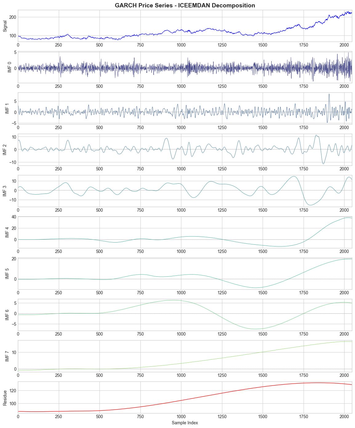
Signal: Simulated GARCH(1,1) price series exhibiting volatility clustering — note the increased fluctuations around samples 1800-2000.

IMF	Frequency	Trading Interpretation
IMF 0	Highest	Market microstructure noise, bid-ask bounce. Amplitude scales with volatility.
IMF 1	High	Tick-level noise, HFT activity. Still shows volatility clustering.
IMF 2	Medium-High	Intraday oscillations, mean-reversion at short scales.
IMF 3	Medium	Swing patterns, ~10-15 bar cycles. Short-term momentum.
IMF 4-5	Low	Multi-day/week cycles. Institutional rebalancing, options expiry effects.
IMF 6-7	Very Low	Monthly/quarterly cycles. Earnings, macro regimes.
Residue	Trend	Underlying drift component.

Each IMF captures roughly half the frequency of the previous, octave-spaced bands without manual tuning.

---

Trading Application: Denoising

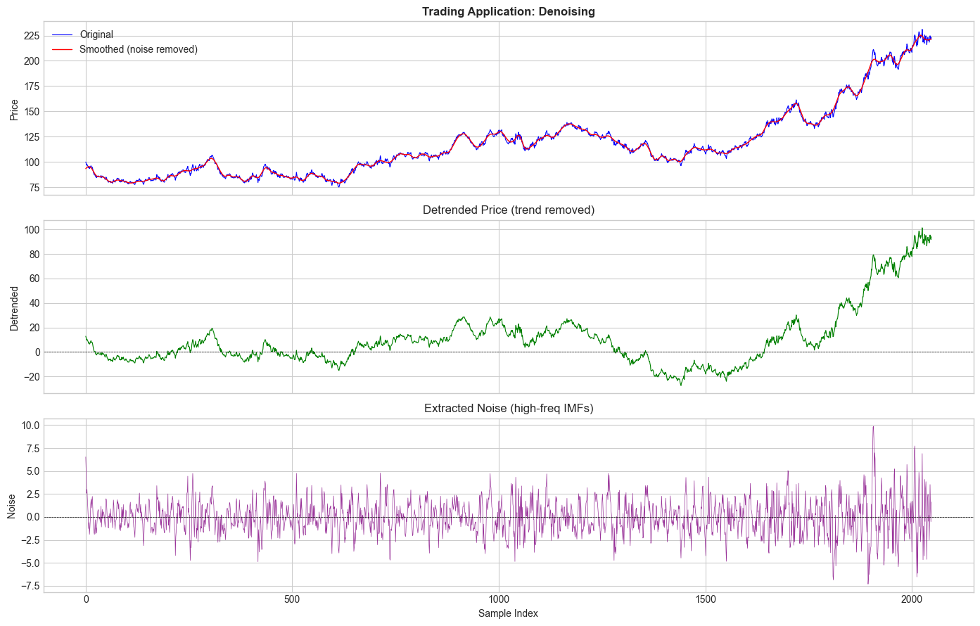
Top: Original price (blue) vs smoothed (red) with high-frequency IMFs removed — ideal for trend-following.

Middle: Detrended price oscillates around zero — suitable for mean-reversion strategies.

Bottom: Extracted noise (IMF 0-1). Note the heteroskedasticity — amplitude increases during high-vol regimes (samples 1500-2000). For volatility estimation, this “noise” is the signal.

---

Reconstruction Verification

Proof that ICEEMDAN is a complete decomposition: ∑IMFs + Residue = Original Signal.

• Max error: 3×10⁻⁸ (machine precision)
• No information loss: Selectively reconstruct using any IMF subset

---

3D Hilbert Spectrum

Time-frequency energy distribution via Hilbert-Huang Transform.

• Yellow region: Trend component, >95% of energy
• Terraced ridges: Clean frequency separation per IMF
• Energy bulge at t=1500-2000: GARCH volatility clustering visible across all bands
• 1/f decay: Characteristic pink noise structure of financial markets

---

Quick Start

Prerequisites

• C++17 compiler (GCC 9+, Clang 10+, MSVC 2019+, Intel ICX)
• Intel oneAPI MKL (free download from Intel)
• CMake 3.20+

Installation

git clone https://github.com/yourusername/iceemdan-mkl.git
cd iceemdan-mkl
cmake -B build -DCMAKE_BUILD_TYPE=Release
cmake --build build

Basic Usage

#include "iceemdan_mkl.hpp"

int main() {
    // Your signal data
    std::vector<double> signal(1024);
    // ... fill signal ...
    
    // Decompose
    eemd::ICEEMDAN decomposer;
    std::vector<std::vector<double>> imfs;
    std::vector<double> residue;
    
    decomposer.decompose(signal.data(), signal.size(), imfs, residue);
    
    // imfs[0] = highest frequency component
    // imfs[n-1] = lowest frequency component
    // residue = trend
    
    return 0;
}

Processing Modes

Three built-in modes optimize for different use cases:

Standard Mode (Default)

Best for: Audio processing, seismic analysis, biomedical signals

eemd::ICEEMDAN decomposer;  // Standard mode by default
// or explicitly:
eemd::ICEEMDAN decomposer(eemd::ProcessingMode::Standard);

• Cubic splines (smooth C² interpolation)
• Global volatility scaling
• Mirror boundary extension

Scientific Mode

Best for: Research requiring reproducibility and audit trails

eemd::ICEEMDAN decomposer(eemd::ProcessingMode::Scientific);
decomposer.config().rng_seed = 42;  // Fixed seed for reproducibility

eemd::DecompositionDiagnostics diag;
decomposer.decompose_with_diagnostics(signal, n, imfs, residue, diag);

// Audit trail
std::cout << "Seed used: " << diag.rng_seed_used << "\n";
std::cout << "Orthogonality index: " << diag.orthogonality_index << "\n";

• Cubic splines
• No variance reduction tricks (pure algorithm)
• Full convergence tracking

Finance Mode

Best for: Quantitative trading, real-time analysis

eemd::ICEEMDAN decomposer(eemd::ProcessingMode::Finance);

// Features:
// - Akima splines (outlier-resistant, no overshoot on gaps/crashes)
// - EMA volatility scaling (adapts to regime changes)
// - AR(1) boundary extrapolation (causal, no look-ahead)
// - NaN/Inf sanitization (handles bad data feeds)
// - Convergence tracking

Why Akima splines for finance?

Standard cubic splines are smooth but “overshoot” on sharp price moves (flash crashes, earnings gaps). This creates phantom high-frequency oscillations in IMF 1-2 that don’t exist in the data.

Akima splines use local 5-point slope estimation — they’re virtually immune to distant outliers:

Spline	Continuity	Behavior on Gaps	Best For
Cubic	C² (smooth)	Overshoots	Smooth signals
Akima	C¹ (local)	Tight, stable	Financial data
Linear	C⁰	No overshoot	Very sparse extrema

Configuration

Common Parameters

eemd::ICEEMDAN decomposer;
auto& cfg = decomposer.config();

cfg.ensemble_size = 100;      // Number of noise realizations (default: 100)
cfg.noise_std = 0.2;          // Noise amplitude as fraction of signal std (default: 0.2)
cfg.max_imfs = 10;            // Maximum IMFs to extract (default: 10)
cfg.max_sift_iters = 100;     // Sifting iterations per IMF (default: 100)
cfg.sift_threshold = 0.05;    // Sifting convergence threshold (default: 0.05)
cfg.rng_seed = 42;            // Random seed for reproducibility (default: 0 = random)

Spline Methods

Controls envelope interpolation:

// Cubic: Smooth C² spline (default for Standard/Scientific)
cfg.spline_method = eemd::SplineMethod::Cubic;

// Akima: Local C¹ spline, outlier-resistant (default for Finance)
cfg.spline_method = eemd::SplineMethod::Akima;

// Linear: Simple linear interpolation (fastest, for very sparse extrema)
cfg.spline_method = eemd::SplineMethod::Linear;

Note: Akima requires minimum 5 data points and strict geometric constraints. If these aren’t met, the implementation automatically falls back to Cubic splines for that envelope — no manual handling needed.

Volatility Methods

Controls how noise is scaled across the signal:

// Global: Single std-dev (fastest, good for stationary signals)
cfg.volatility_method = eemd::VolatilityMethod::Global;

// SMA: Rolling window std-dev (adapts to local variance)
cfg.volatility_method = eemd::VolatilityMethod::SMA;
cfg.vol_window = 100;  // Lookback window

// EMA: Exponential moving std-dev (fastest adaptation)
cfg.volatility_method = eemd::VolatilityMethod::EMA;
cfg.vol_ema_span = 20;  // EMA span

Boundary Methods

Controls extrapolation at signal edges:

// Mirror: Reflects extrema (smooth, slight look-ahead)
cfg.boundary_method = eemd::BoundaryMethod::Mirror;

// AR: Autoregressive extrapolation (causal, no look-ahead)
cfg.boundary_method = eemd::BoundaryMethod::AR;
cfg.ar_damping = 0.5;  // 0=mean-revert, 1=full AR

// Linear: Simple linear extrapolation
cfg.boundary_method = eemd::BoundaryMethod::Linear;

Algorithm Details

ICEEMDAN vs EEMD vs EMD

Method	Mode Mixing	Completeness	Computation
EMD	Severe	Complete	Fast
EEMD	Reduced	Incomplete	Slow
CEEMDAN	Reduced	Complete	Slow
ICEEMDAN	Minimal	Complete	Slow

ICEEMDAN adds noise to the residue at each stage (not the original signal), producing cleaner IMFs with better frequency separation.

S-Number Sifting Criterion

In addition to the standard SD (stopping difference) criterion, this implementation uses the S-number criterion for faster convergence:

cfg.s_number = 6;  // Stop after 6 consecutive iterations with stable extrema count

When the number of extrema remains unchanged for S iterations, the IMF is considered converged. This provides ~15% speedup with identical decomposition quality. Set to 0 to disable.

Orthogonality Index

Lower is better. Measures mode mixing:

eemd::DecompositionDiagnostics diag;
decomposer.decompose_with_diagnostics(signal, n, imfs, residue, diag);
std::cout << "IO: " << diag.orthogonality_index << "\n";  // Good: < 0.1

IMF Interpretation

IMF 1: Highest frequency oscillations
IMF 2: Second highest frequency
...
IMF N: Lowest frequency oscillations  
Residue: Monotonic trend

For analysis:

// Hurst exponent (persistence)
// H < 0.5: Mean-reverting
// H = 0.5: Random walk
// H > 0.5: Trending

// Compute instantaneous frequency via Hilbert transform
// (not included, use your preferred implementation)

Examples

Detrending a Signal

eemd::ICEEMDAN decomposer;
decomposer.decompose(signal, n, imfs, residue);

// Detrended = signal - residue
std::vector<double> detrended(n);
for (int i = 0; i < n; ++i) {
    detrended[i] = signal[i] - residue[i];
}

Extracting Specific Frequency Bands

decomposer.decompose(signal, n, imfs, residue);

// High-frequency component (first few IMFs)
std::vector<double> high_freq(n, 0.0);
for (int k = 0; k < 3; ++k) {
    for (int i = 0; i < n; ++i) {
        high_freq[i] += imfs[k][i];
    }
}

// Low-frequency component (remaining IMFs + residue)
std::vector<double> low_freq(n, 0.0);
for (int k = 3; k < imfs.size(); ++k) {
    for (int i = 0; i < n; ++i) {
        low_freq[i] += imfs[k][i];
    }
}
for (int i = 0; i < n; ++i) {
    low_freq[i] += residue[i];
}

Reconstruction Verification

// IMFs + residue should exactly reconstruct the signal
std::vector<double> reconstructed(n, 0.0);
for (const auto& imf : imfs) {
    for (int i = 0; i < n; ++i) {
        reconstructed[i] += imf[i];
    }
}
for (int i = 0; i < n; ++i) {
    reconstructed[i] += residue[i];
}

// Verify
double max_error = 0.0;
for (int i = 0; i < n; ++i) {
    max_error = std::max(max_error, std::abs(signal[i] - reconstructed[i]));
}
std::cout << "Reconstruction error: " << max_error << "\n";  // Should be ~1e-15

Finance Mode with Akima Splines

eemd::ICEEMDAN decomposer(eemd::ProcessingMode::Finance);

// Finance mode automatically sets:
// - spline_method = Akima (with Cubic fallback)
// - volatility_method = EMA
// - boundary_method = AR (causal)
// - sanitize_input = true

decomposer.decompose(prices, n, imfs, residue);

// IMF 0-1: Market microstructure noise
// IMF 2-3: Short-term mean-reversion
// IMF 4+: Swing/trend components
// Residue: Long-term drift

Benchmarking

Build and run the benchmarks:

./build/iceemdan_bench         # General performance
./build/iceemdan_finance_bench # Finance-specific tests
./build/bench_snumber          # S-number optimization benchmark

Visualization (Jupyter Notebook)

Generate CSV files and visualize with Python:

# 1. Build and run CSV export example
cmake -B build -DCMAKE_BUILD_TYPE=Release
cmake --build build
./build/example_finance_csv

# 2. Open Jupyter notebook
cd jupyter
jupyter notebook iceemdan_visualization.ipynb

The notebook shows:

• Full decomposition plots (signal + all IMFs + residue)
• Energy distribution across IMFs
• Reconstruction verification
• Frequency analysis per IMF
• Trading applications (detrending, denoising)

References

1. ICEEMDAN: Colominas, M. A., Schlotthauer, G., & Torres, M. E. (2014). Improved complete ensemble EMD: A suitable tool for biomedical signal processing. Biomedical Signal Processing and Control, 14, 19-29.

2. CEEMDAN: Torres, M. E., Colominas, M. A., Schlotthauer, G., & Flandrin, P. (2011). A complete ensemble empirical mode decomposition with adaptive noise. ICASSP 2011.

3. EEMD: Wu, Z., & Huang, N. E. (2009). Ensemble empirical mode decomposition: a noise-assisted data analysis method. Advances in Adaptive Data Analysis, 1(01), 1-41.

4. EMD: Huang, N. E., et al. (1998). The empirical mode decomposition and the Hilbert spectrum for nonlinear and non-stationary time series analysis. Proceedings of the Royal Society A, 454(1971), 903-995.

5. Akima Splines: Akima, H. (1970). A new method of interpolation and smooth curve fitting based on local procedures. Journal of the ACM, 17(4), 589-602.

Citation

If you use this implementation in your research, please cite:

@software{iceemdan_mkl,
  author = Tugbars Heptaskin,
  title = {ICEEMDAN-MKL: High-Performance ICEEMDAN Implementation},
  year = {2025},
  url = {https://github.com/Tugbars/iceemdan-mkl}
}

License

MIT License. See LICENSE for details.

Contributing

Contributions welcome! Please open an issue or PR.

Acknowledgments

• Intel MKL for high-performance spline fitting
• Original ICEEMDAN algorithm by Colominas et al.
• Akima spline method for robust envelope construction